Notes / G.01
From light transport to samples.
Path tracing estimates the rendering equation by sampling random light paths; dividing each contribution by its sampling density keeps the estimate unbiased, while finite samples appear as noise.
01 / Mental model
Follow energy backward from the camera.
A camera ray finds a surface, then recursively samples where the arriving light may have come from. Visibility, emission, material response, and geometry determine how much of that energy reaches the pixel.
02 / Core mechanism
The rendering equation becomes an estimator.
Outgoing radiance combines emitted light with reflected incoming radiance over the surface hemisphere.
Monte Carlo integration replaces the continuous integral with weighted samples. A better sampling distribution reduces variance without changing the expected result.
03 / Implementation
Keep the estimator explicit.
- Generate a primary camera ray and intersect the scene.
- Sample a direction from the BSDF and retain its probability density.
- Accumulate throughput across bounces; stop on a miss or an emitter.
- Use Russian roulette for long paths and average samples progressively in linear color.
04 / Evidence
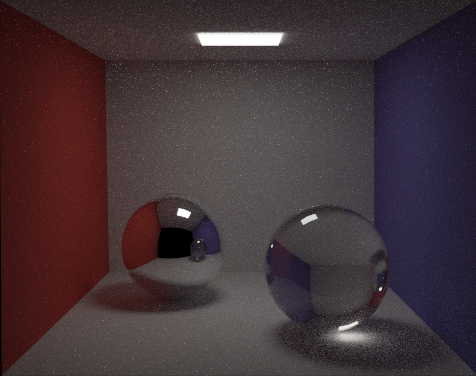
Read the image as a diagnostic.
Noise should decrease with more samples while the mean remains stable. Soft shadows, indirect illumination, and color bleeding show that multi-bounce transport is present; persistent bias or fireflies point back to sampling and weighting choices.